Browsing waveforms with the WaveformBrowser
This is a tutorial demonstrating several ways to use the WaveformBrowser to examine waveform data. This will consist of multiple examples, increasing in complexity, and will use LEGEND test data from pylegendtestdata. The WaveformBrowser [docs] is a dspeed utility for accessing waveforms from raw files in an interactive way,
enabling you to access, draw, or even process waveforms. Some use cases for this utility include investigating a population of waveforms, and debugging waveform processors.
Why do we need a waveform browser when we can access data via Pandas dataframes? Pandas dataframes work extremely well for reading tables of simple values from multiple HDF5 files. However, they are less optimal for waveforms. The reason for this is that they require holding all waveforms in memory at once. If we want to look at waveforms spread out across multiple files, this can potentially take up GBs of memory, which will cause problems! To get around this, we want to load only bits of the
files into memory at a time and pull out only what we need. Since this is an inconvenient process, the WaveformBrowser will do this for you, while hiding the details as much as possible.
Let’s start by importing necessary modules and test data:
[1]:
%matplotlib inline

import matplotlib.pyplot as plt
import pandas as pd
import numpy as np
import os, json
import pint

u = pint.get_application_registry()

import lh5
from dspeed.vis.waveform_browser import WaveformBrowser
from legendtestdata import LegendTestData

ldata = LegendTestData()
raw_file = ldata.get_path("lh5/LDQTA_r117_20200110T105115Z_cal_geds_raw.lh5")

plt.rcParams["figure.figsize"] = (14, 4)
plt.rcParams["figure.facecolor"] = "white"
plt.rcParams["font.size"] = 14
Basic browsing
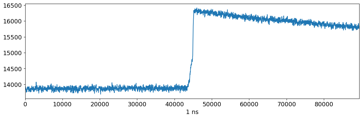
First, a minimal example simply drawing waveforms from the raw file. Let’s create a minimal browser and draw the 50th waveform:
[2]:
browser = WaveformBrowser(raw_file, "geds/raw")
browser.draw_entry(50)
Found waveforms dict_keys(['waveform']). Use the lines argument to select one or more.
To draw multiple waveforms in a single figure, provide a list if indices:
[3]:
browser.draw_entry([64, 82, 94])

Now draw the next waveform in the file. You can run this cell multiple times to scroll through many waveforms:
[4]:
browser.draw_next();

Filtering waveforms
Ok, that was nice, but how often do we just want to scroll through all of our waveforms?
For our next example, we will select a population of waveforms from within the files, and draw multiple at once. Selecting a population of events to draw uses the same syntax as NumPy and Pandas, and can be done either with a list of entries or a boolean NumPy array. This selection can be made using data from a DSP file (or higher tiers).
We will also learn how to set a few other properties of the figure.
Let’s quickly produce a DSP file (see tutorial on running DSP):
[5]:
from dspeed import build_dsp

dsp_file = "LDQTA_r117_20200110T105115Z_cal_geds_dsp.lh5"
build_dsp(
    raw_file, dsp_out=dsp_file, dsp_config="metadata/dsp-config.json", write_mode="r"
)
Now, we load a Pandas DataFrame from the file that we can use to make our selection:
[6]:
from lh5 import read_as

df = read_as("geds/dsp", dsp_file, "pd", field_mask=["trapEmax", "AoE"])
display(df)
| AoE | trapEmax | |
|---|---|---|
| 0 | 0.047916 | 2485.666504 |
| 1 | 0.022737 | 6708.169922 |
| 2 | 0.072955 | 6923.642578 |
| 3 | 0.075722 | 9795.389648 |
| 4 | 0.031047 | 2855.946289 |
| ... | ... | ... |
| 95 | 0.073018 | 2924.060303 |
| 96 | 0.030934 | 2804.429443 |
| 97 | 0.045665 | 28556.371094 |
| 98 | 0.045562 | 4559.607422 |
| 99 | 0.045889 | 2572.662109 |
100 rows × 2 columns
We use Pandas’ querying syntax to create a selection mask around high energy events:
[7]:
energy = df["trapEmax"]
energy_selection = (energy > 10000) & (energy < 30000)
Let’s have a look at them:
[8]:
energy.hist(bins=200, range=(0, 30000))
energy[energy_selection].hist(bins=200, range=(0, 30000))
plt.xlabel("energy [a.u.]");

We then construct a WaveformBrowser with this cut:
[9]:
browser = WaveformBrowser(
    raw_file,
    "geds/raw",
    aux_values=df,
    legend="E = {trapEmax}",  # values to put in the legend
    x_lim=(40 * u.us, 50 * u.us),  # range for time-axis
    entry_mask=energy_selection,  # apply cut
    n_drawn=5,  # number to draw for draw_next
)
Found waveforms dict_keys(['waveform']). Use the lines argument to select one or more.
And finally draw the next 5 batches of 10 waveforms:
[10]:
for entries, i in zip(browser, range(2)):
    browser.new_figure()


If you can use interactive plots, you can replace browser.new_figure() with e.g. plt.pause(1) to draw a slideshow!
Visualizing waveform transforms
Now, we’ll shift from drawing populations of waveforms to drawing waveform transforms. We can draw any waveforms that are defined in a DSP JSON configuration file. This is useful for debugging purposes and for developing processors. We will draw the baseline subtracted waveform, pole-zero corrected waveform, and trapezoidal filter waveform. We will also draw horizontal and vertical lines for trapE (the maximum of the trapezoid) and tp_0 (our estimate of the start of the waveform’s rise).
The browser will determine whether these lines should be horizontal or vertical based on the unit.
[11]:
browser = WaveformBrowser(
    raw_file,
    "geds/raw",
    dsp_config="metadata/dsp-config.json",  # Need to include a dsp config file!
    database={"pz_const": "180*us"},
    lines=[
        "wf_blsub",
        "wf_pz",
        "wf_trap",
        "trapEmax",
        "tp_0",
    ],  # names of waveforms from dsp config file
    styles=[
        {"ls": ["-"], "c": ["orange"]},
        {"ls": [":"], "c": ["green"]},
        {"ls": ["--"], "c": ["blue"]},
        {"lw": [0.5], "c": ["black"]},
        {"lw": [0.5], "c": ["red"]},
    ],
    legend=[
        "Waveform",
        "PZ Corrected",
        "Trap Filter",
        "Trap Max = {trapEmax}",
        "t0 = {tp_0}",
    ],
    legend_opts={"loc": "upper left"},
    x_lim=("35*us", "75*us"),  # x axis range
)
[12]:
browser.draw_next();

Comparing waveforms
Here’s a more advanced example that combines the previous two. We will draw waveforms from multiple populations for the sake of comparison. This will require creating two separate browsers and drawing them onto the same axes. We’ll also normalize and baseline-subtract the waveforms from parameters in a DSP file. Finally, we’ll add some formatting options to the lines and legend.
We start by selecting two sub-populations from the high-energy events from above by cutting on A/E:
[13]:
aoe = df["AoE"]
aoe_cut = (aoe < 0.045) & energy_selection
aoe_accept = (aoe > 0.045) & energy_selection

aoe[aoe_accept].hist(bins=200, range=(0, 0.1))
aoe[aoe_cut].hist(bins=200, range=(0, 0.1))
plt.xlabel("A/E [a.u.]");

Now, we create two distinct browsers:
[14]:
browser1 = WaveformBrowser(
    raw_file,
    "geds/raw",
    dsp_config="metadata/dsp-config.json",
    lines="wf_blsub",  # draw baseline subtracted waveform instead of the original
    norm="trapEmax",  # normalize waveforms based on amplitude
    styles={"color": ["red", "orange"]},  # set a color cycle for this
    legend="E = {trapEmax} ADC, A/E = {AoE:~.3f}",  # formatted values to put in the legend
    x_lim=(40 * u.us, 50 * u.us),
    entry_mask=aoe_cut,  # apply the first cut
    n_drawn=2,
)
browser2 = WaveformBrowser(
    raw_file,
    "geds/raw",
    dsp_config="metadata/dsp-config.json",
    lines="wf_blsub",
    norm="trapEmax",
    styles={"color": ["blue", "cyan"]},
    legend="E = {trapEmax} ADC, A/E = {AoE:~.3f}",
    legend_opts={
        "loc": "lower right",
        "bbox_to_anchor": (1, 0),
    },  # set options for drawing the legend
    x_lim=(40 * u.us, 50 * u.us),
    entry_mask=aoe_accept,  # apply the other cut
    n_drawn=2,
)
/home/docs/checkouts/readthedocs.org/user_builds/dspeed/envs/stable/lib/python3.10/site-packages/dspeed/processing_chain.py:1780: RuntimeWarning: invalid value encountered in divide
  self.processor(*self.args, **self.kwargs)
And draw!
[15]:
browser1.draw_next()
browser2.set_figure(browser1)  # use the same figure/axis as the other browser
browser2.draw_next(clear=False);  # Set clear to false to draw on the same axis!

Direct access of waveforms and other quantities
The waveforms, lines and legend entries are all stored inside of the waveform browser. Sometimes you want to access these directly; maybe you want to access the raw data, or do control the lines in a way not enabled by the WaveformBrowser interface. It is possible to access them quickly and easily.
When accessing waveforms in this way, you can also do the same things previously shown, such as applying a data cut and grabbing processed waveforms. For this example, we are going to get waveforms, trap-waveforms and trap energies, after applying an A/E cut.
Let’s start by defining a browser object:
[16]:
browser = WaveformBrowser(
    raw_file,
    "geds/raw",
    dsp_config="metadata/dsp-config.json",
    database={"pz_const": "180*us"},
    lines=["waveform", "wf_trap"],
    legend=["E = {trapEmax}"],
    entry_mask=aoe_accept,
    n_drawn=2,
)
Waveforms and legend values are stored as a dictionary from the parameter name to a list of stored values:
The waveforms are as a list of matplotlib
Line2DartistsHorizontal and vertical lines are also stored as
Line2DartistsLegend entries are stored as pint
Quantities
Now, let’s simply print them:
[17]:
browser.find_next()
waveforms = browser.lines["waveform"]
traps = browser.lines["wf_trap"]
energies = browser.legend_vals["trapEmax"]
for wf, trap, en in zip(waveforms, traps, energies):
    print("Raw waveform:", wf.get_ydata())
    print("Trap-filtered waveform:", trap.get_ydata())
    print("TrapEmax:", en)
    print()
Raw waveform: [11538. 11538. 11608. ... 23720. 23653. 23629.]
Trap-filtered waveform: [-0.14880781 -0.29762885 -0.33446312 ... 29.209356   29.145533
 29.009712  ]
TrapEmax: 15478.6669921875

Raw waveform: [16610. 16610. 16578. ... 28694. 28775. 28751.]
Trap-filtered waveform: [ 0.19340937  0.38683593  0.5290797  ... 51.572906   51.32965
 51.11198   ]
TrapEmax: 15687.3857421875
This page has been automatically generated by nbsphinx and can be run as a Jupyter notebook available in the dspeed repository.