DSP Tutorial

So, You Want to Add a Signal Processing Routine

This tutorial will teach you multiple ways to write signal processing routines, incorporate them into a data analysis, and run that data analysis.

OUTLINE: we will write a set of processors to measure the current of our waveforms. The processors will be written to demonstrate a variety of patterns used when writing processors for use in dspeed. After this, we will show how to incorporate these into the signal processing framework of dspeed.

Section I: Writing processors 1) ufuncs as processors: BL mean and BL subtraction using numpy 2) numba guvectorize to write ufuncs: pole-zero 3) non-trivial numba: decrease size of output: derivative 4) object mode for wrapping other processors: gaussian convolution 5) factory method for processors that require initialization: triangle convolution

Section II: Creating and running a processing chain 1) Making a json file 2) Running build_dsp (link to other DSP tutorial) 3) Running WaveformBrowser (link to WB tutorial, show only simple example)

Before we begin, some setup…

%matplotlib inline

import os, json
import matplotlib.pyplot as plt
import numpy as np

from lgdo import lh5
from legendtestdata import LegendTestData

# Get some sample waveforms from LEGEND test data
ldata = LegendTestData()
raw_file = ldata.get_path("lh5/LDQTA_r117_20200110T105115Z_cal_geds_raw.lh5")
st = lh5.LH5Store()
tab = st.read("geds/raw", raw_file)[0]
wfs = tab["waveform"].values.nda.astype("float32")
t = tab["waveform"].dt.nda.reshape((100, 1)) * np.arange(wfs.shape[1])
baselines = tab["baseline"].nda

# Set up default plot style
plt.rcParams["figure.figsize"] = (14, 4)
plt.rcParams["figure.facecolor"] = "white"
plt.rcParams["font.size"] = 14

Part I: Processing data in bulk using ufuncs

Universal functions, or ufuncs, operate on numpy ndarrays in an element-wise fashion. Ufuncs have several features that make them valuable for signal processing: 1) Vectorized: ufuncs operate on full arrays, element-by-element. This is much faster (in python) than manually looping over the array, and may enable hardware optimizations to speed up code 2) Broadcasting: ufuncs can automatically figure out the size and type of an output array based on the inputs to the function, making them flexible and easy to use 3) In place operations: ufuncs can store their output in pre-allocated memory, reducing the need for allocating/de-allocating arrays, which is an expensive operation

For example, we can subtract the baseline from each of our waveforms as follows:

wf_blsub = np.zeros_like(wfs)
np.subtract(wfs, baselines.reshape((len(baselines), 1)), out=wf_blsub);

Our original waveforms:

plt.plot(t[0:10].T, wfs[0:10].T);

Our processed waveforms:

plt.plot(t[0:10].T, wf_blsub[0:10].T);

Woohoo, it worked! And it applied to all of our waveforms (since it is vectorized)! Even though there is a single baseline value for each of our length 5592 waveforms, broadcasting caused the correct value to be subtracted from every waveform sample, producing a (100, 5592) to match the input. Also note that we predefined our output wf_blsub and operated on it in place rather than creating a new array.

Creating a simple processor with numba.guvectorize

While ufuncs are powerful and can be combined to do lots of things, sometimes we want to break beyond the confines of the existing ufuncs and write more complex processors. For this, we use numba, which will convert your python code into C and just-in-time (JIT) compile it for improved performance. In particular, we will use guvectorize to write generalized ufuncs (gufuncs).

These gufuncs have the same advantageous properties that we outlined above for ufuncs, namely that they are vectorized, allow for broadcasting, and can operate in place. However, gufuncs have additional flexibility since they can be broadcast over arrays rather than just elements. In other words, they are not constrained to perform the same operation on each element of an array, and can instead be programmed to perform the same operation over sub-arrays. This is controlled by specifying the signature of the gufunc.

To illustrate how this works, we will write a guvectorized processor that pole-zero corrects our waveforms to remove the exponential decay on the tails:

* Note, that there are recommended conventions for writing gufuncs to be included in dspeed, which are outlined at the end of this tutorial. For simplicity and illustrative purposes, we ignore these for now

from numba import guvectorize


@guvectorize(["(float32[:], float32, float32[:])"], "(n),()->(n)", nopython=True)
def polezero(w_in: np.ndarray, tau: float, w_out: np.ndarray):
    const = np.exp(-1 / tau)
    w_out[0] = w_in[0]
    for i in range(1, len(w_in), 1):
        w_out[i] = w_out[i - 1] + w_in[i] - w_in[i - 1] * const

Let’s walk through what that does:

• @guvectorize “decorates” the python function we define, causing it to produce a JIT-compiled function instead of a normal python function

• ["(float32[:], float32, float32[:])"] defines the the data types of the input arguments. In this case, we take an array of floats, a scalar float, and output an array of floats. Note that if the output is a scalar, we must still use the array notation [:] to ensure that the value can be changed in-place. Also note that multiple sets of inputs may be specified. (This is very similar to the C convention of passing pointers to variables/arrays so that we can change them inside of a function. Just replace the pointer symbol * with the array [:]!)

• "(n),()->(n)" defines the “signature” of the function, which specifies the sub-arrays that we define our operation over. In this case, we supply a vector of length n, a scalar, and output a vector of length n. When we input arrays into our function, these are the right-most dimension, and it is important that the length of this dimension matches (i.e. w_in and w_out must have the same length). The function will implicitly broadcast over any additional dimensions (meaning we can supply arrays with >1 dimension). Type signatures can get more complex than this by employing additional characters to describe dimensions (e.g. matrix multiplication would look like (m,n),(n,p)->(m,p)).

• nopython=True tells numba to use JIT-compilation to produce speedier code. Alternatively, we can supply forceobj=True to not JIT-compile things and instead just vectorize python code. This can be useful for wrapping functions from other libraries, as we will see later.

• def polezero(w_in: np.ndarray, tau: float, w_out: np.ndarray):: the definition of our function. This must have the same number of arguments as our signature and data types. The last argument w_out is our output. Note that the function can be run out-of-place by not supplying an argument, which will cause it to allocate and return a new array. The type annotations are not necessary, but are recommended for readability.

• for i in range(1, len(w_in), 1): In the definition of our function, we use a loop. This is notable, because in base-python we ordinarily want to avoid loops for high-performance code. In this case, because numba is JIT-compiling C-code, however, this loop will perform very well.

Now we will try out our function:

wf_pzcorr = np.zeros_like(wfs)
polezero(wf_blsub, 10000, out=wf_pzcorr)
plt.plot(t[0:10].T, wf_pzcorr[0:10].T);

Huzzah, the decay has been removed from the tails!

Now, we will present some other examples, that utilize more advanced features of numba.

Advanced guvectorize: changing shape of output

Sometimes, the output of a processor will differ in size from the inputs. For example, this occurs often when doing convolutions, derivatives, or changing the sampling period of a waveform. As an example, we will implement a derivative using finite-difference across n_samp points:

@guvectorize(["(float32[:], float32[:])"], "(n),(m)", nopython=True)
def derivative(w_in: np.ndarray, w_out: np.ndarray):
    n_samp = len(w_in) - len(w_out)
    for i_samp in range(len(w_out)):
        w_out[i_samp] = w_in[i_samp + n_samp] - w_in[i_samp]

Some important differences between this and our “basic” example:

• "(n),(m)": notice that we are not using -> to denote that w_out is an output. That is because numba only let’s us define new signature sizes for inputs, since it cannot deduce m from the other inputs. This means that we must be careful about specifying the length of our output waveform when we allocate it. This also means that this processor will only work in-place!

• n_samp = len(w_in) - len(w_out): also notice that we did not feed n_samp as an input, but instead calculate it inside of the function.

Now, let’s test it out:

# set n_samp and use it to shape our output array
n_samp = 5
wf_deriv = np.zeros((wfs.shape[0], wfs.shape[1] - n_samp), "float32")

derivative(wf_blsub, wf_deriv)
plt.plot(t[0:10, n_samp // 2 : -n_samp // 2].T, wf_deriv[0:10].T)
plt.xlim(42000, 48000);

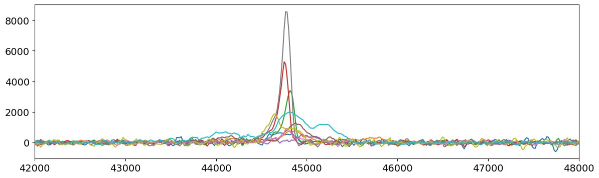
Yippee, now we have current pulses!

Advanced guvectorize: wrapping functions from other python libraries

Often, someone will have already written a well-optimized function to apply whatever processor we want. In this case, rather than reimplementing the function in numba, we can simply write a wrapper for it. As we will soon see, it is often not necessary (or optimal) to wrap a function in this way, but we will write an example for demonstration purposes. We will wrap scipy’s gaussian_filter1D:

from scipy.ndimage import gaussian_filter1d


@guvectorize(["(float32[:], float32, float32[:])"], "(n),()->(n)", forceobj=True)
def gauss_filter(w_in: np.ndarray, sigma: float, w_out: np.ndarray):
    gaussian_filter1d(w_in, sigma, output=w_out, mode="nearest")

The important difference between this and our “basic” example:

forceobj=True: instead of using nopython mode, which causes numba to convert our function to C and compile it, forceobj mode executes the function in python, after wrapping it in the gufunc interface. This makes the function vectorized, and enables broadcasting; this interface also makes plugging the function into the dspeed framework very simple (see below). However, as noted above, it is not always necessary or desirable to do this; if a function is already vectorized, wrapping it can be redundant (this is actually the case for the above example). When using forceobj mode, we lose the advantages of nopython, such as faster loops.

Now, let’s test it out:

wf_deriv_gauss = np.zeros_like(wf_deriv)
gauss_filter(wf_deriv, 3, wf_deriv_gauss)
plt.plot(t[0:10, n_samp // 2 : -n_samp // 2].T, wf_deriv_gauss[0:10].T)
plt.xlim(42000, 48000);

Boo-yah! Look how smooth that is!

Advanced guvectorize: writing a function that can be initialized

Sometimes, we need to be able to provide extra steps that are used to set up a processor. For example, we may want to read in values from a file, or compute a convolution kernel. Often, supplying these as arguments to the function is cumbersome, so instead we apply the “factory” technique.

The “factory” technique entails writing a python function that performs this setup, compiles a numbified function, and then returns that function so that we can apply it to waveforms. In the following example, we will use this method to construct a triangular convolution kernel and apply it to our waveform.

def triangle_filter(length: int):
    # build triangular kernel
    kernel = np.concatenate(
        [
            np.arange(1, length // 2 + 1, dtype="f"),
            np.arange((length + 1) // 2, 0, -1, dtype="f"),
        ]
    )
    kernel /= np.sum(kernel)  # normalize

    @guvectorize(["(float32[:], float32[:])"], "(n)->(n)", forceobj=True, cache=False)
    def returned_filter(w_in: np.ndarray, w_out: np.ndarray):
        w_out[:] = np.convolve(w_in, kernel, mode="same")

    return returned_filter

What’s happening here?

• When we call the outer function triangle_filter, is is building a convolution kernel, and then having numba generate a gufunc that will convolve the input with this kernel. The returned function has this kernel hard-coded into it (meaning the kernel is not an argument and cannot be changed without re-calling triangle_filter to generate a new gufunc).

• cache=False: by setting cache=True, we can tell numba to store a copy of the function to disk. This is not something we want with factory functions, since we want to make copies that are different from one another!

wf_deriv_tri = np.zeros_like(wf_deriv)
tri_filter = triangle_filter(10)
tri_filter(wf_deriv, wf_deriv_tri)

plt.plot(t[0:10, n_samp // 2 : -n_samp // 2].T, wf_deriv_tri[0:10].T)
plt.xlim(42000, 48000);

Hot dog, those are some smooth current pulses!

Conventions for writing dspeed processors

In order to produce consistently styled, readable code with well-defined behaviors for errors, we follow several conventions (see documentation here)

from dspeed.errors import DSPFatal
from dspeed.utils import numba_defaults_kwargs as nb_kwargs


@guvectorize(
    ["void(float32[:], float32, float32[:])", "void(float64[:], float64, float64[:])"],
    "(n),()->(n)",
    **nb_kwargs,
)
def pole_zero(w_in: np.ndarray, t_tau: float, w_out: np.ndarray) -> None:
    """Apply a pole-zero cancellation using the provided time
    constant to the waveform.

    Parameters
    ----------
    w_in
        the input waveform.
    t_tau
        the time constant of the exponential to be deconvolved.
    w_out
        the pole-zero cancelled waveform.

    JSON Configuration Example
    --------------------------

    .. code-block :: json

        "wf_pz": {
            "function": "pole_zero",
            "module": "dsp_tutorial",
            "args": ["wf_bl", "400*us", "wf_pz"],
            "unit": "ADC"
        }
    """
    if np.isnan(t_tau) or t_tau == 0:
        raise DSPFatal("t_tau must be a non-zero number")

    w_out[:] = np.nan

    if np.isnan(w_in).any():
        return

    const = np.exp(-1 / t_tau)
    w_out[0] = w_in[0]
    for i in range(1, len(w_in), 1):
        w_out[i] = w_out[i - 1] + w_in[i] - w_in[i - 1] * const

• Type signatures: we tend to prefer floating point types, since these can be set to NaN (not-a-number, see below). Only use other types if you know this will not be an issue. We usually create 2 versions of the type signature, one for 32-bit and one for 64-bit

• variable naming conventions: for waveforms use w_[descriptor]; for timepoints use t_[descriptor]; for amplitude values use a_descriptor

• nb_kwargs: we encode many of the options for guvectorize in nb_kwargs. Default values are determined using the environment variables described here. For example, we set nopython = True using these defaults. To override defaults, do nb_kwargs( arg=val )

• Docstring: use the scikit-hep style. In addition, add an example JSON block to add the processor (see below).

• NaNs: for undefined behavior and errors associated with individual waveforms, our preferred approach is to set outputs to NaN, or not-a-number, (and to propagate NaNs to future processor outputs). Typically, we begin by defaulting outputs to NaN, and apply NaN checks to inputs before we begin the processor

Finally, let’s write a python module, tutorial_procs, containing each of our numbafied functions, written in the dspeed style. A module file created in this way can be installed so that it can be used by dspeed’s DSP framework, as we will see below.

Part II: Using dspeed to combine multiple processors

We’ve just learned how to create DSP transforms; now we will see how to combine these into a single data analysis using the dspeed ProcessingChain. ProcessingChain is an object that reads data from LH5 files, applies a sequence of processors, and then outputs the results into a new LH5 file. There are several advantages to using ProcessingChain:

• Manages memory and file I/O for you in an efficient way

• Performs unit conversions for you, so that you can apply unit-less processors

• Automatically* deduces the properties (i.e. shapes, dtypes, units) of variables

• Set up using portable, easy-to-use JSON files

The remainder of this tutorial will show you how to build a JSON file to setup a processing chain, how to use that to process an LH5 file, and how to interactively view each step of the analysis using the WaveformBrowser. We will be building a python dictionary, but it is very easy to translate this into a json file. Broadly speaking, the structure we use to define our processors is:

"processors": {
    "[name of parameter(s)]": {
        "function": "[name of function]",
        "module": "[python module containing function]",
        "args": [ "names", "of", "args"],
        ... other optional args ...
    }
}

* Automation is never a perfect process; we will see how to override automated choices below

Now, let’s build a JSON config (ok, actually a python dict) for the analysis we did above! For another example of a standard Ge detector analysis, see the Intro to DSP tutorial.

config = {
    "processors": {
        "wf_blsub": {
            "function": "subtract",
            "module": "numpy",
            "args": ["astype(waveform, 'float32')", "baseline", "wf_blsub"],
        }
    }
}

This will call numpy.subtract(waveform, baseline, out=wf_blsub). The ProcessingChain will find waveform and baseline in the input file, and create wf_blsub with the correct shape, data type and units automatically. The ProcessingChain is also capable of parsing certain operations (such as astype or +-+/).

config["processors"].update(
    {
        "wf_pz": {
            "function": "pole_zero",
            "module": "tutorial_procs",
            "args": ["wf_blsub", "625*us", "wf_pz"],
        }
    }
)

This will call the polezero function we wrote above (in typical operation, it is recommended that you write your functions into your own module and import from there). Note that we are defining the PZ-time constant in units of us rather than number of samples! wf_blsub will be autmotically found from our previously defined processor.

config["processors"].update(
    {
        "wf_deriv": {
            "function": "derivative",
            "module": "tutorial_procs",
            "args": ["wf_pz", "wf_deriv(shape = len(wf_pz)-5, period=wf_pz.period)"],
        }
    }
)

This will call the derivative function we wrote above. Note that in this case, we are overriding the automatic decision by ProcessingChain to make wf_deriv and wf_pz the same shape.

config["processors"].update(
    {
        "wf_deriv_gauss": {
            "function": "gauss_filter",
            "module": "tutorial_procs",
            "args": ["wf_deriv", "50*ns", "wf_deriv_gauss"],
        },
        "wf_deriv_tri": {
            "function": "triangle_filter",
            "module": "tutorial_procs",
            "args": ["wf_deriv", "wf_deriv_tri"],
            "init_args": ["160*ns/wf_deriv.period"],
        },
    }
)

Recall that we created triangle_filter using the “factory” method to initialize it during setup. ProcessingChain will read out the initialization parameters from “init_args”.

Finally, we will add a couple of processors to extract the maximum current amplitude from each filter.

config["processors"].update(
    {
        "A_raw": {
            "function": "amax",
            "module": "numpy",
            "args": ["wf_deriv", 1, "A_raw"],
            "kwargs": {"signature": "(n),()->()", "types": ["fi->f"]},
        },
        "A_gauss": {
            "function": "amax",
            "module": "numpy",
            "args": ["wf_deriv_gauss", 1, "A_gauss"],
            "kwargs": {"signature": "(n),()->()", "types": ["fi->f"]},
        },
        "A_tri": {
            "function": "amax",
            "module": "numpy",
            "args": ["wf_deriv_tri", 1, "A_tri"],
            "kwargs": {"signature": "(n),()->()", "types": ["fi->f"]},
        },
    }
)

To extract the current amplitudes, we are calling np.amax, which is not formatted as a ufunc. We can still use it by specifying the shape and type signals, using the “kwargs” entry as above.

The final step to defining our ProcessingChain is to tell it which variables to output to file. The ProcessingChain will ensure that it runs all of the processors necessary to build the output variables (and it will ignore any extraneous processors).

config["outputs"] = ["A_raw", "A_gauss", "A_tri"]

Executing our Processing Chain

Once you have defined a JSON DSP configuration file, you can use it to run build_dsp:

from dspeed import build_dsp

build_dsp(
    f_raw=raw_file,
    f_dsp="test_dsp.lh5",
    dsp_config=config,
    lh5_tables="geds/raw",
    write_mode="o",
)

A command line tool exists for doing this. Equivalently to the above command, you can do:

dspeed build-dsp -o test_dsp.lh5 -g geds/raw -c [config_file].json -w [raw_file].lh5

st = lh5.LH5Store()

lh5.show("test_dsp.lh5")
print()
print(st.read("geds/dsp", "test_dsp.lh5")[0].get_dataframe())

/
└── geds · HDF5 group
    └── dsp · table{A_raw,A_gauss,A_tri}
        ├── A_gauss · array<1>{real}
        ├── A_raw · array<1>{real}
        └── A_tri · array<1>{real}

          A_raw      A_gauss        A_tri
0    640.123901   578.318542   592.716858
1    785.578613   699.859192   728.085938
2   3401.478027  2408.934570  2734.619141
3   5278.631836  3564.308105  4032.437256
4    540.191772   415.844452   435.277802
..          ...          ...          ...
95  1264.582031   997.185791  1063.104858
96   592.171875   429.947693   467.865997
97  6663.067383  6365.070801  6438.286621
98  1526.402344   982.292603  1129.659912
99   751.140503   573.289917   615.581787

[100 rows x 3 columns]

/tmp/ipykernel_984/2162832340.py:5: DeprecationWarning: `get_dataframe` is deprecated and will be removed in a future release. Instead use `view_as` to get the Table data as a pandas dataframe or awkward Array.
  print(st.read("geds/dsp", "test_dsp.lh5")[0].get_dataframe())

Using the waveform browser to look at transforms

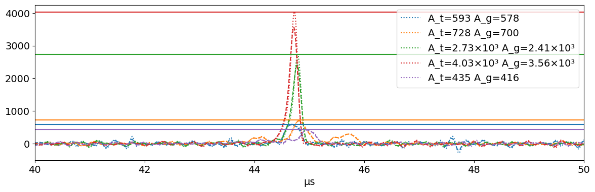
The WaveformBrowser (tutorial here) is a tool meant to enable you to draw waveforms from LH5 data files. This tool is designed to interact with a ProcessingChain, and can be used to view the effects of processors (and debug them as needed).

from dspeed.vis.waveform_browser import WaveformBrowser
import matplotlib.colors as mcolors

print()
browser = WaveformBrowser(
    raw_file,
    "geds/raw",
    dsp_config=config,
    lines=["wf_deriv_tri", "wf_deriv_gauss", "A_tri"],
    styles=[
        {"ls": [":"] * 10, "color": mcolors.TABLEAU_COLORS.values()},
        {"ls": ["--"] * 10, "color": mcolors.TABLEAU_COLORS.values()},
    ],
    legend=["A_t={A_tri} A_g={A_gauss}"],
    x_lim=("40*us", "50*us"),
)

browser.draw_next(5)
plt.show()

---

This page has been automatically generated by nbsphinx and can be run as a Jupyter notebook available in the dspeed repository.