Introduction to Digital Signal Processing

This notebook will provide a brief introduction to a few of LEGEND’s bread and butter digital signal processing filters. These processors will be applied in sequence to digitized waveforms that are recorded to disk, and a brief explanation of why we use them is provided. The parameters of each processor may be varied as well in order to see the affects that they have.

Recommended reading is Radiation Detection and Measurement by Glenn F. Knoll, Chapter 17, which introduces many pulse-shaping concepts (although, from a hardware-perspective more than a digital signal processing perspective; even so, the concepts are similar).

Set up the Python environment

It is recommended that you use a file from the LEGEND test-data repository; you may need to change data_file if you want to run this notebook yourself. We use the Python wrapper of the test-data repository.

from lh5 import read, read_as, ls, show
from dspeed.vis import WaveformBrowser
from dspeed import units
from dspeed import build_dsp

import matplotlib.pyplot as plt
import os
from legendtestdata import LegendTestData

ldata = LegendTestData()
data_file = ldata.get_path("lh5/LDQTA_r117_20200110T105115Z_cal_geds_raw.lh5")
entry_no = 2  # which waveform in our example data_file to use for plotting

plt.rcParams["figure.figsize"] = (14, 4)
plt.rcParams["figure.facecolor"] = "white"
plt.rcParams["font.size"] = 12

Processor Setup

This next panel defines all of the processors that we are going to run. Normally this is done in a JSON file in almost the exact same format shown here [here’s a detailed specification]. You are encouraged to try changing some of the values in these processors to see the effect on the analysis.

dsp_config = {
    "outputs": [
        "timestamp",
        "channel",
        "trapEmax",
        "trapTmax",
        "tp_0",
        "ftp",
        "trapEftp",
        "bl",
        "bl_sig",
        "A_gaus",
    ],
    "processors": {
        "max_index": {
            "function": "argmax",
            "module": "numpy",
            "args": ["waveform", 1, "max_index"],
            "kwargs": {"signature": "(n),()->()", "types": ["fi->i"]},
            "unit": "ADC",
        },
        "bl, bl_sig, slope, intercept": {
            "function": "linear_slope_fit",
            "module": "dspeed.processors",
            "args": ["waveform[:1650]", "bl", "bl_sig", "slope", "intercept"],
            "unit": ["ADC", "ADC", "ADC", "ADC"],
        },
        "wf_blsub": {
            "function": "subtract",
            "module": "numpy",
            "args": ["waveform", "bl", "wf_blsub"],
            "unit": "ADC",
        },
        "wf_pz": {
            "function": "pole_zero",
            "module": "dspeed.processors",
            "args": ["wf_blsub", "180*us", "wf_pz"],
            "unit": "ADC",
        },
        "wf_trap": {
            "function": "trap_norm",
            "module": "dspeed.processors",
            "args": ["wf_pz", "8*us", "2*us", "wf_trap"],
            "unit": "ADC",
        },
        "trapEmax": {
            "function": "amax",
            "module": "numpy",
            "args": ["wf_trap", 1, "trapEmax"],
            "kwargs": {"signature": "(n),()->()", "types": ["fi->f"]},
            "unit": "ADC",
        },
        "trapTmax": {
            "function": "argmax",
            "module": "numpy",
            "args": ["wf_trap", 1, "trapTmax"],
            "kwargs": {"signature": "(n),()->()", "types": ["fi->i"]},
            "unit": "ns",
        },
        "wf_atrap": {
            "function": "asym_trap_filter",
            "module": "dspeed.processors",
            "args": [
                "wf_pz",
                "0.1*us",
                "1*us",
                "3*us",
                "wf_atrap",
            ],  # rising edge, flat section, falling edge
            "unit": "ADC",
        },
        "tmax": {
            "function": "argmax",
            "module": "numpy",
            "args": ["wf_atrap", 1, "tmax"],
            "kwargs": {"signature": "(n),()->()", "types": ["fi->i"]},
            "unit": "ns",
        },
        "tp_0": {
            "function": "time_point_thresh",
            "module": "dspeed.processors",
            "args": ["wf_atrap", 0, "tmax", 0, "tp_0"],
            "unit": "ns",
        },
        "ftp": {
            "function": "add",
            "module": "numpy",
            "args": ["tp_0", "2*us+8*us-256*ns", "ftp"],
            "unit": "ns",
        },
        "trapEftp": {
            "function": "fixed_time_pickoff",
            "module": "dspeed.processors",
            "args": ["wf_trap", "ftp", "105", "trapEftp"],  # ord('i') == 105
            "unit": "ADC",
        },
        "curr": {
            "function": "avg_current",
            "module": "dspeed.processors",
            "args": ["wf_pz", 1, "curr(len(wf_pz)-1, 'f', period=waveform.period)"],
            "unit": "ADC/sample",
        },
        "gaus_kernel": {
            "function": "gaussian_filter1d",
            "module": "dspeed.processors",
            "args": ["50", "4", "gaus_kernel(shape=401, dtype='d')"],
        },
        "curr_gaus": {
            "function": "reflected_convolve_wf",
            "module": "dspeed.processors",
            "args": [
                "curr",
                "gaus_kernel",
                "curr_gaus(len(curr), 'f', period=waveform.period)",
            ],
            "unit": "ADC/sample",
        },
        "A_gaus": {
            "function": "amax",
            "module": "numpy",
            "args": ["curr_gaus", 1, "A_gaus"],
            "kwargs": {"signature": "(n),()->()", "types": ["fi->f"]},
            "unit": "ADC/sample",
        },
    },
}

Plotting Processors via WaveformBrowser

In the next cells, we will use the WaveformBrowser [docs] function to visualize the various processors that are calculated in the config file. See the WaveformBrowser tutorial for more info.

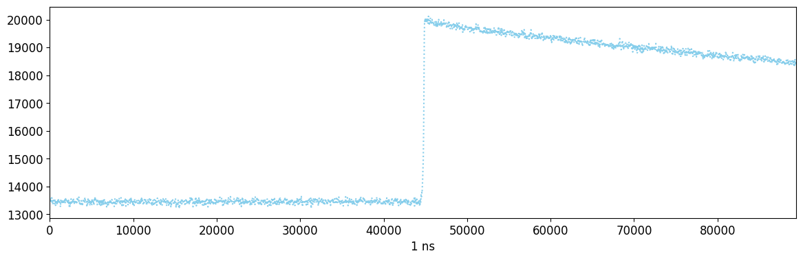
Raw Waveform

This is a waveform as produced by a flashcam digitizer. The waveform can be divided into three regions; first, the baseline, the flat part up to ~45000 ns. Next the rising edge, where it increases at ~45000 ns. Lastly, the falling tail, which is an approximately exponential return to baseline that begins after ~45000 ns.

Note that, in the below, we do not specify the lines keyword argument, as is done in subsequent cells. The default behavior in this case is to plot the raw waveform.

browser = WaveformBrowser(
    data_file,
    "geds/raw",
    styles=[
        {"color": ["skyblue"], "ls": ["dotted"]},
    ],
)
browser.draw_entry(entry_no)

Found waveforms dict_keys(['waveform']). Use the lines argument to select one or more.

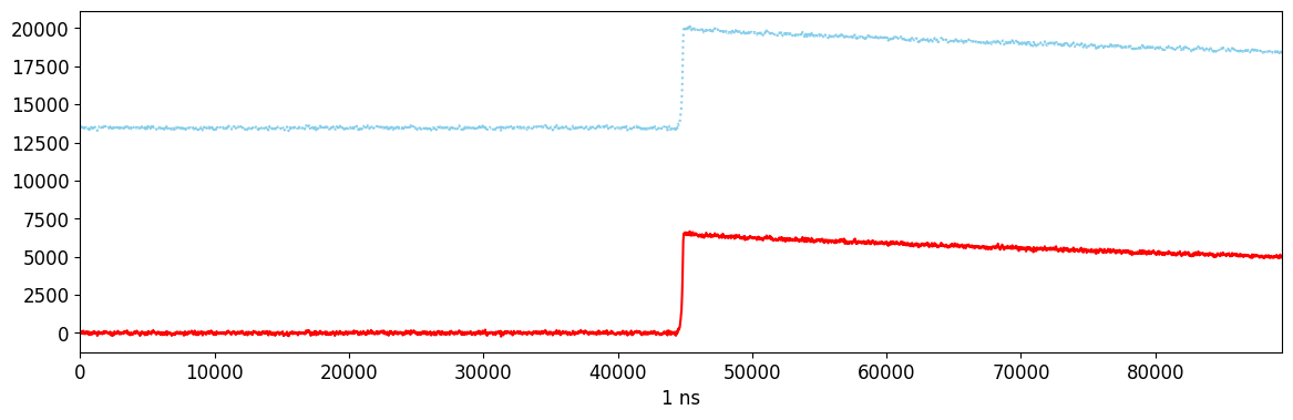
Baseline Subtraction

The first processors applied perform baseline subtraction. First we measure the baseline using the first 1650 samples of the waveform, and then we subtract the baseline from each sample.

browser = WaveformBrowser(
    data_file,
    "geds/raw",
    dsp_config=dsp_config,
    lines=["waveform", "wf_blsub"],
    styles=[
        {"color": ["skyblue"], "ls": ["dotted"]},
        {"color": ["r"]},
    ],
)
browser.draw_entry(entry_no)

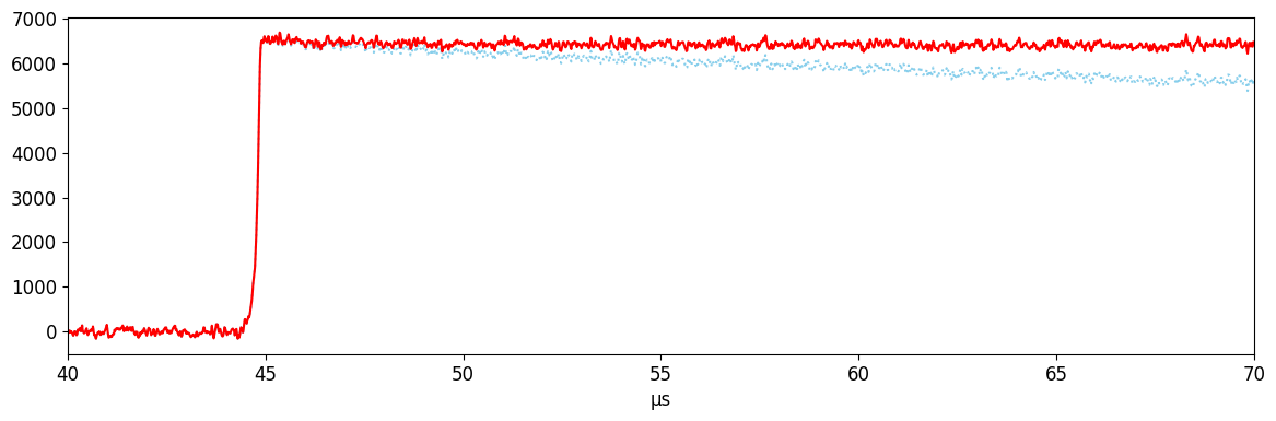
Pole-Zero Correction

The next step is to correct our waveform for the electronics response, which produces the exponential shape characteristic of our waveforms. The goal of this transform is to return a waveform with a perfectly flat tail. The pole-zero correction assumes a simple electronics response characterized by a single RC constant (in this case 180 microseconds). In reality, our electronics can be characterized by multiple RC constants; as a result we do not achieve a perfectly flat top, but by applying more complex transforms at this step we can improve things. The pole-zero applied here is close enough for most applications, though.

Knoll chapter 17 sec. 7B gives a more complete description.

browser = WaveformBrowser(
    data_file,
    "geds/raw",
    dsp_config=dsp_config,
    lines=["wf_blsub", "wf_pz"],
    styles=[
        {"color": ["skyblue"], "ls": [":"]},
        {"color": ["r"]},
    ],
    x_lim=("40*us", "70*us"),
)
browser.draw_entry(entry_no)

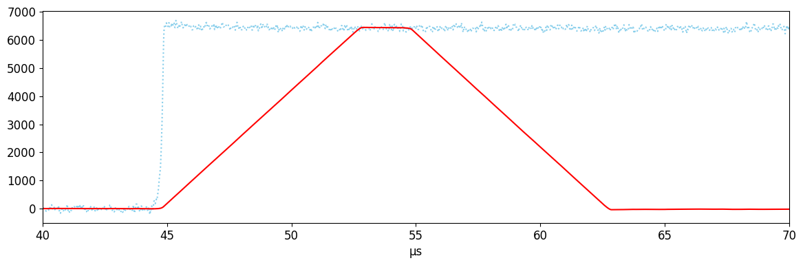
Trapezoidal Filter

The trapezoidal filter is a nearly optimal filter that is used to extract pulse amplitude for a variety of applications. The trapezoid is the difference, at each point, between the average over two sets of samples separated by a short time. It can be characterized by:

• Integration time: number of samples averaged, and the length of the rising and falling edges of the trapezoid. We use 8 microseconds here. A longer integration time will reduce the effect of noise on our energy measurement (up to a limit that depends on low frequency noise; it also can’t be too long for the number of samples collected).

• Flat top time: the separation between the integration regions, and the length of the flat top of the trapezoid. This should be longer than the rising edge of the waveform; if it is not, the top will not be totally flat and we will measure a reduction in the charge called “ballistic deficit.” We also don’t want the flat top to be too long, or else low frequency noise will degrade our resolution. Here, we use 2 us as our flat top time.

Knoll Chapter 17 Sec. 7 has a description of trapezoidal shaping.

browser = WaveformBrowser(
    data_file,
    "geds/raw",
    dsp_config=dsp_config,
    lines=["wf_pz", "wf_trap"],
    styles=[
        {"color": ["skyblue"], "ls": [":"]},
        {"color": ["r"]},
    ],
    x_lim=("40*us", "70*us"),
)
browser.draw_entry(entry_no)

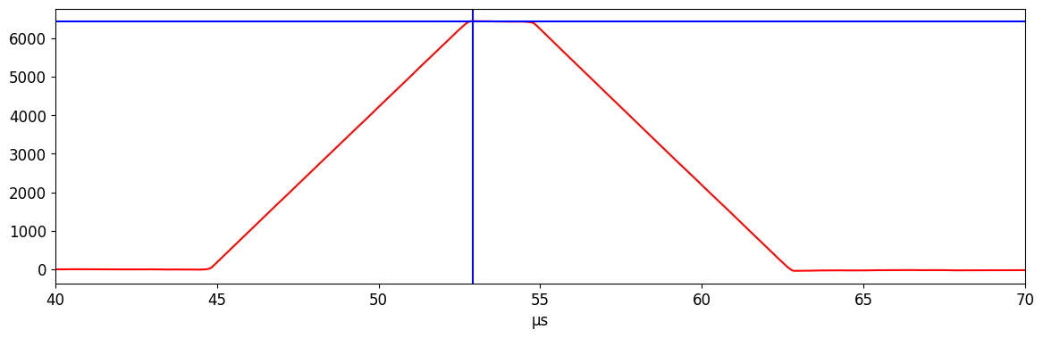
Energy estimation: trap-max

The most common way to measure uncalibrated energy is to use the maximum of the trapezoidal filter. This works fairly well, assuming you have a nice flat top; however, due to our imperfect pole-zero correction, this can result in a degradation in our energy resolution.

browser = WaveformBrowser(
    data_file,
    "geds/raw",
    dsp_config=dsp_config,
    lines=["wf_trap", "trapEmax", "trapTmax"],
    styles=[
        {"color": ["r"]},
        {"color": ["b"]},
        {"color": ["b"]},
    ],
    x_lim=("40*us", "70*us"),
)
browser.draw_entry(entry_no)

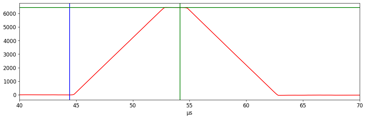
Energy estimation: fixed time pick-off

Another way to measure energy is to pick-off the amplitude of the trapezoidal filter at a fixed time relative to the start of the waveform. The fixed time should fall on the flat top of the waveform, with enough padding to avoid ballistic deficit, and to prevent noise in the start time from pushing the pick-off time onto the falling edge of the waveform. We choose a pickoff time 0.25 microseconds before the falling edge begins. This technique also requires an accurate measurement of the start time (\(t_0\)) of the waveform (see next section).

browser = WaveformBrowser(
    data_file,
    "geds/raw",
    dsp_config=dsp_config,
    lines=["wf_trap", "tp_0", "ftp", "trapEftp"],
    styles=[
        {"color": ["r"]},
        {"color": ["b"]},
        {"color": ["g"]},
        {"color": ["g"]},
    ],
    x_lim=("40*us", "70*us"),
)
browser.draw_entry(entry_no)

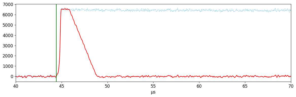
Start time measurement

The start time (\(t_0\)) of the waveform must be measured in order to apply the fixed-time pickoff. We use the following technique to measure this:

1. Apply an asymmetric trapezoidal filter, which uses a short integration time for the rising edge and a long integration time for the falling tail. The short rising edge has the advantage of preserving most timing information in the rising edge. The longer tail helps us correct for low frequency noise. Here, we use 0.1 / 1 / 3 microseconds as the rise / flat / fall times.

2. Find the maximum of the asymmetric-trap, and walk back from there until we cross zero. The first sample that we cross this threshold is our \(t_0\).

An accurate \(t_0\) is important both for the fixed-time pickoff, and for various drift-time corrections (such as for charge-trapping) that are not described in this notebook. While this filter is mostly reliable, it can occasionally fail for low signal-to-noise waveforms, or waveforms with large transiant blips in the noise.

browser = WaveformBrowser(
    data_file,
    "geds/raw",
    dsp_config=dsp_config,
    lines=["wf_pz", "wf_atrap", "tp_0"],
    styles=[
        {"color": ["skyblue"], "ls": [":"]},
        {"color": ["r"]},
        {"color": ["g"]},
    ],
    x_lim=("40*us", "70*us"),
)
browser.draw_entry(entry_no)

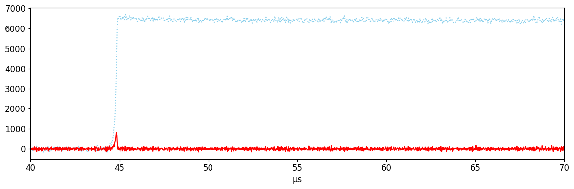
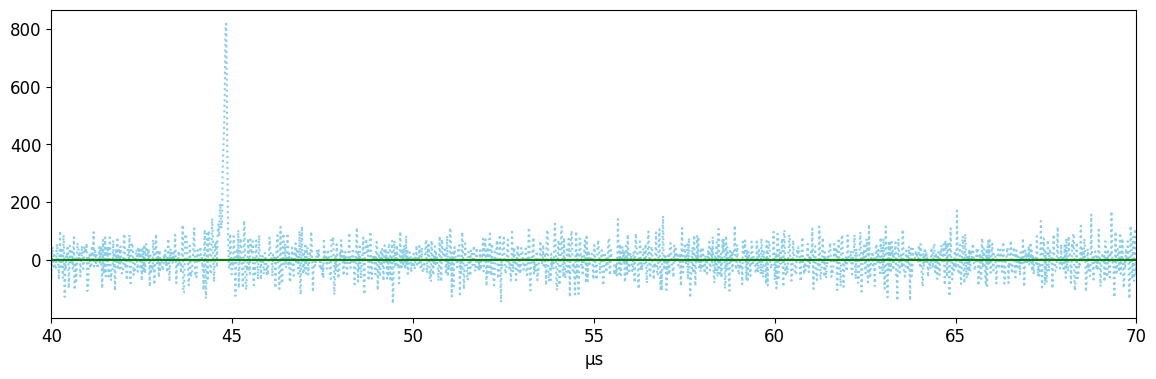
Current measurement

Current is needed to measure \(A/E\). This can be found using a simple derivative filter. However, the signal-to-noise using just the derivative can be quite high, so we often apply additional smoothing filters after (see next section).

browser = WaveformBrowser(
    data_file,
    "geds/raw",
    dsp_config=dsp_config,
    lines=[
        "wf_pz",
        "curr",
    ],
    styles=[
        {"color": ["skyblue"], "ls": [":"]},
        {"color": ["r"]},
    ],
    x_lim=("40*us", "70*us"),
)
browser.draw_entry(entry_no)

Gaussian-smoothed current

One way we can improve the signal-to-noise ratio is by applying a gaussian filter. This is a convolution of our waveform with a gaussian kernel. While this reduces the impact of noise on our measurement, it also reduces the timing information in the rising edge, reducing the signal; as a result, we must find an optimal balance in our smoothing. Knoll chapter 17 Sec. 4 describes gaussian shaping.

The current amplitude (\(A\)) is the maximum of the smoothed current waveform.

browser = WaveformBrowser(
    data_file,
    "geds/raw",
    dsp_config=dsp_config,
    lines=["curr", "curr_gaus", "A_gaus"],
    styles=[{"color": ["skyblue"], "ls": [":"]}, {"color": ["r"]}, {"color": ["g"]}],
    x_lim=("40*us", "70*us"),
)
browser.draw_entry(entry_no)

Using build_dsp()

At this point, we have used the WaveformBrowser to view the outputs of the various DSP calculations that were specified in our example dsp_config from earlier. However, we have not actually saved these outputs to any file. In dspeed, this is done via the build_dsp() [docs] function, which takes our raw example file, runs the processing chain, and saves the outputs to a new LH5 file, which we will simply name example_dsp_file.lh5.

Let’s build the DSP!

build_dsp(
    data_file,
    dsp_out="./example_dsp_file.lh5",
    dsp_config=dsp_config,
    write_mode="r",  # used to overwrite an existing file
)

We can now take a look at the contents of the new file, using either ls() [docs] or show() [docs] from lh5 [docs]. Working with LH5 files is discussed in further detail in the LH5Files tutorial, and we direct the reader there for more information.

ls("example_dsp_file.lh5")

['geds']

show("example_dsp_file.lh5")

/
└── geds · struct{dsp}
    └── dsp · table{A_gaus,bl,bl_sig,channel,ftp,timestamp,tp_0,trapEftp,trapEmax,trapTmax}
        ├── A_gaus · array<1>{real}
        ├── bl · array<1>{real}
        ├── bl_sig · array<1>{real}
        ├── channel · array<1>{real}
        ├── ftp · array<1>{real}
        ├── timestamp · array<1>{real}
        ├── tp_0 · array<1>{real}
        ├── trapEftp · array<1>{real}
        ├── trapEmax · array<1>{real}
        └── trapTmax · array<1>{real}

We see that we have indeed saved our output values in dsp_config to this new file. Lastly, let’s access them to see the actual values, again as similarly done in the LH5Files tutorial.

obj = read("geds/dsp", "./example_dsp_file.lh5")
print(
    f"We have saved the following list of outputs from our DSP routine: {list(obj.keys())}"
)
print(
    f"There are {len(obj)} rows of values, corresponding to that same number of waveforms."
)

We have saved the following list of outputs from our DSP routine: ['A_gaus', 'bl', 'bl_sig', 'channel', 'ftp', 'timestamp', 'tp_0', 'trapEftp', 'trapEmax', 'trapTmax']
There are 100 rows of values, corresponding to that same number of waveforms.

We see that the various outputs are in this file, and they have been calculated for 100 waveforms.

To manipulate the various values, it is recommended to convert to a Pandas DataFrame, via the provided read_as [docs] function, as show below. We load all of the outputs of the processors to a single DataFrame, specified by inputting the 'geds/dsp' group in the LH5 file.

read_as("geds/dsp", "./example_dsp_file.lh5", "pd")

	A_gaus	bl	bl_sig	channel	ftp	timestamp	tp_0	trapEftp	trapEmax	trapTmax
0	0.0	13720.968750	94.490707	53	54336.0	0.794660	44592.0	2310.669189	2319.071777	52944
1	0.0	13050.674805	50.100597	60	53168.0	0.796899	43424.0	5678.894531	5761.768555	53824
2	0.0	13453.005859	65.760880	40	54160.0	0.799604	44416.0	6428.772461	6439.731445	52912
3	0.0	11828.862305	64.085381	41	54000.0	0.799604	44256.0	9124.365234	9147.147461	52816
4	0.0	14342.213867	46.583649	60	53152.0	0.801617	43408.0	2672.938965	2672.945312	53136
...	...	...	...	...	...	...	...	...	...	...
95	0.0	27145.410156	437.696960	53	54352.0	0.965948	44608.0	3191.124023	3199.575684	52880
96	0.0	14568.882812	49.303154	60	53056.0	0.971051	43312.0	2631.415527	2636.029541	53232
97	0.0	15455.618164	90.539101	53	54320.0	0.973319	44576.0	26523.931641	26580.843750	53024
98	0.0	9922.455078	73.784843	30	54160.0	0.974689	44416.0	4229.133301	4232.768066	54448
99	0.0	16977.902344	85.741364	53	54256.0	0.978621	44512.0	2385.685791	2387.285156	53216

100 rows × 10 columns

And from here, the user can plot various values, manipulate them in some way, or anything else.

---

This page has been automatically generated by nbsphinx and can be run as a Jupyter notebook available in the dspeed repository.